1 Designing a Survey

##Target Population## Define the Target Population In designing an aquatic resource monitoring survey, the designer must define what aquatic resource is to be monitored, otherwise known as the Target Population. For example, if the designer only has an interest in assessing the condition of perennial waters in a state, the target population is defined as perennial waters and intermittent and ephemeral waters are defined as non-target populations and are omitted from the selection process. The target population should align with your organizations monitoring strategy and objectives.

##Sample Frame## Select a Sample Frame of the Target Population Next, the designer must select a Sample Frame to use when selecting potential sampling sites. A sample frame is a GIS representation (e.g. shapefile) of the aquatic resource target population such as National Hydrography Datasets. In the example above, the designer will select a dataset which only includes perennial waters. This process often involves extracting a subset of a dataset which contains non-target resources.

Illustration of a sample frame is constructed

Sample frames for NARS and states may differ due to different target populations, source material, and state knowledge leading to improvements. For partners to leverage NARS fully, requesting the integration of a partners sample frame can possibly be accommodated.

Illustration of a partner sample frame integration

##Prepare a Survey## Once the target population has been defined and a sample frame of the target population has been selected, the designer can now prepare a survey. The code below shows how a survey was designed using a population of lakes in the Northeast US. This sample frame is found in the package spsurvey and is not meant for use other than as an example.

NOTE To upload your own sample frame, you may use the code below to read a file as an sf_object which is required by spsurvey to design a survey.

library(sf)

#Example to read a shapefile
my_sample_frame <- st_read("path/to/my/sample/frame.shp")

#Load the spsurvey package
library(spsurvey)

#To view the NE_Lakes sf object which contains the target population
NE_Lakes <- spsurvey::NE_Lakes

#Plot NE_Lakes 
plot(NE_Lakes, 
     pch = 19,
     main= "NE Lakes",
     key.width = lcm(3))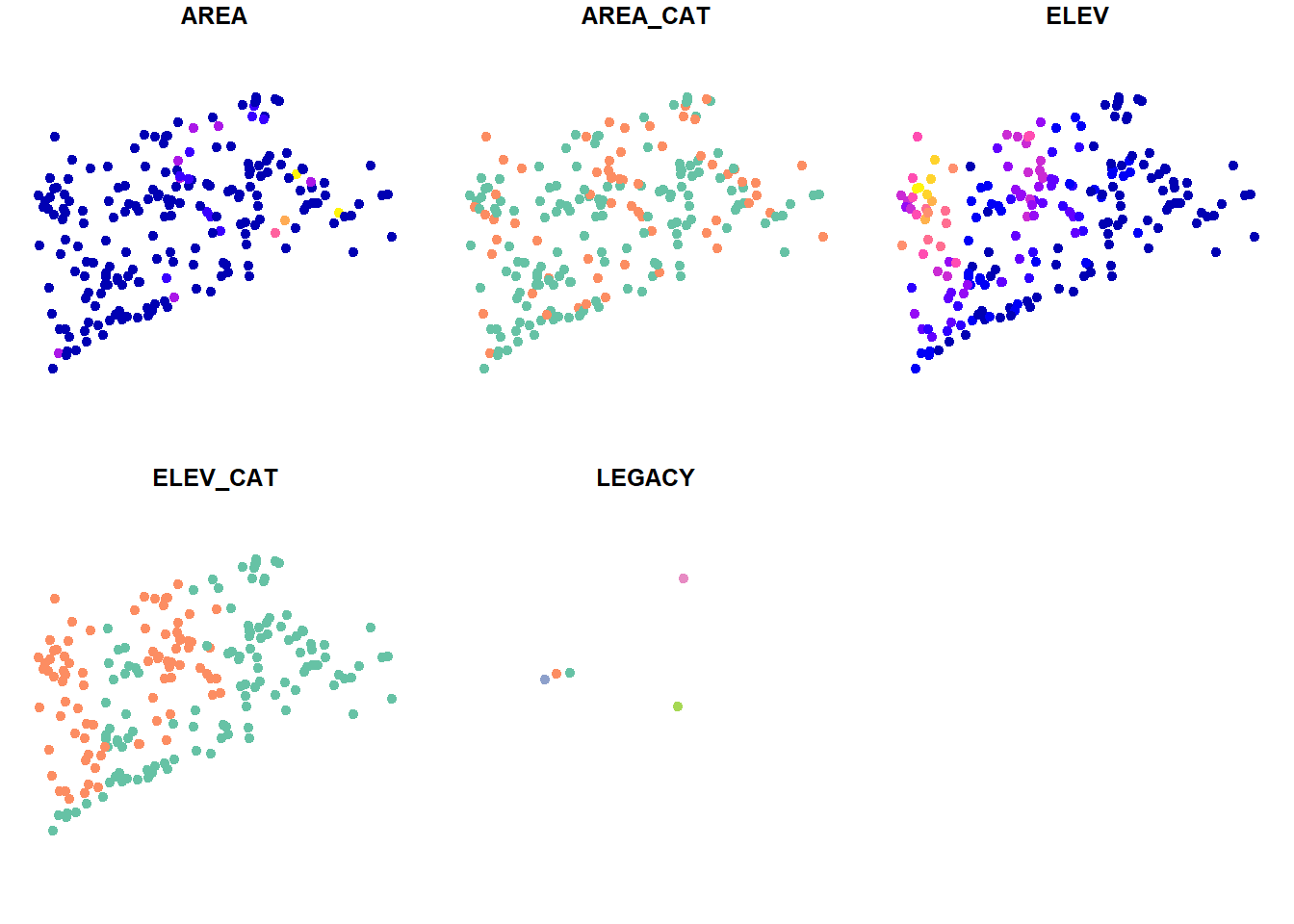

##Unstratified Equal Probablity Design## For a state scale monitoring survey, it is generally accepted that sampling 50 sites gives sufficient confidence when calculating condition estimates. This sample size can vary depending on the size of the sample frame. Below we prepare an unstratified equal probability survey in which all lakes in the sample frame have the same chance of being selected regardless of size or other attributes.

EQ_PROB <- grts(
  NE_Lakes,
  n_base = 50
)

plot(
  EQ_PROB,
  NE_Lakes,
  main= "Base Sample Sites",
  pch = 19,
  key.width = lcm(3)
)

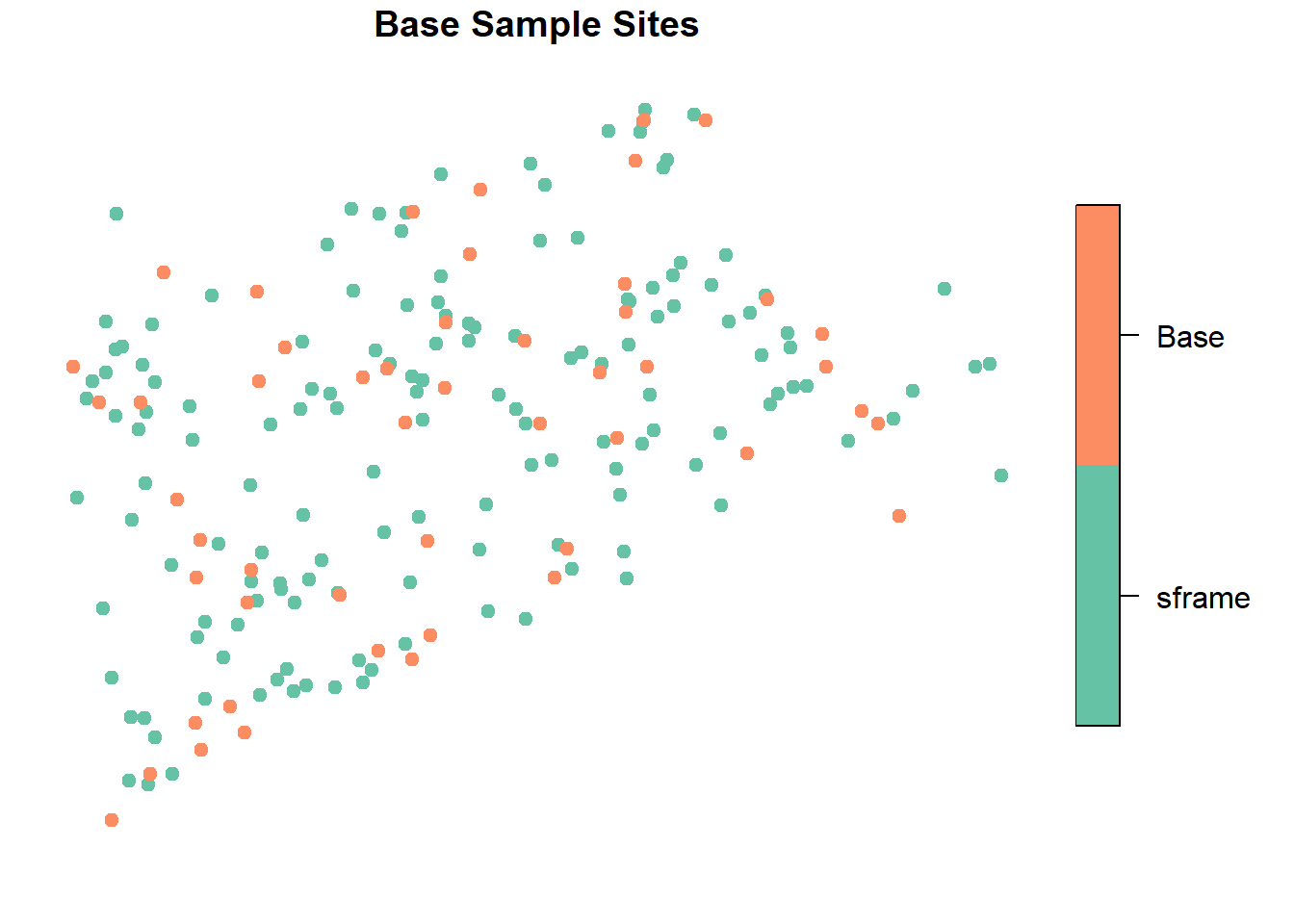
Above, the plot displays the survey sites selected within the sample frame. Use the function spsurvey::sprbind() to obtain the information about each survey site.

#Binds survey site 
EQ_PROB_INFO <- sprbind(EQ_PROB)

#View the first 5 rows
head(EQ_PROB_INFO, 5)

## Simple feature collection with 5 features and 14 fields
## Geometry type: POINT
## Dimension:     XY
## Bounding box:  xmin: 1855254 ymin: 2278764 xmax: 2006131 ymax: 2357507
## Projected CRS: NAD83 / Conus Albers
##    siteID siteuse replsite lon_WGS84 lat_WGS84 stratum wgt   ip caty      AREA
## 1 Site-01    Base     None -72.59874  41.53708    None   4 0.25 None  4.928180
## 2 Site-02    Base     None -73.11579  41.90821    None   4 0.25 None  1.214076
## 3 Site-03    Base     None -73.16363  42.20213    None   4 0.25 None  1.495233
## 4 Site-04    Base     None -71.42052  41.77149    None   4 0.25 None  6.659393
## 5 Site-05    Base     None -72.50852  41.35677    None   4 0.25 None 10.312968
##   AREA_CAT   ELEV ELEV_CAT LEGACY                geometry
## 1    small 150.88     high   <NA> POINT (1918363 2296508)
## 2    small 385.96     high   <NA> POINT (1866906 2326514)
## 3    small 397.62     high   <NA> POINT (1855254 2357507)
## 4    small   6.75      low   <NA> POINT (2006131 2346237)
## 5    large  84.68      low   <NA> POINT (1930547 2278764)

##Proporitional Probablity Design## Often, designers may want to proportionally stratify sites based on a Category.

#Creates an sframe object of northeast lakes found in the spsurvey package
NE_Lakes <- sframe(NE_Lakes)
 
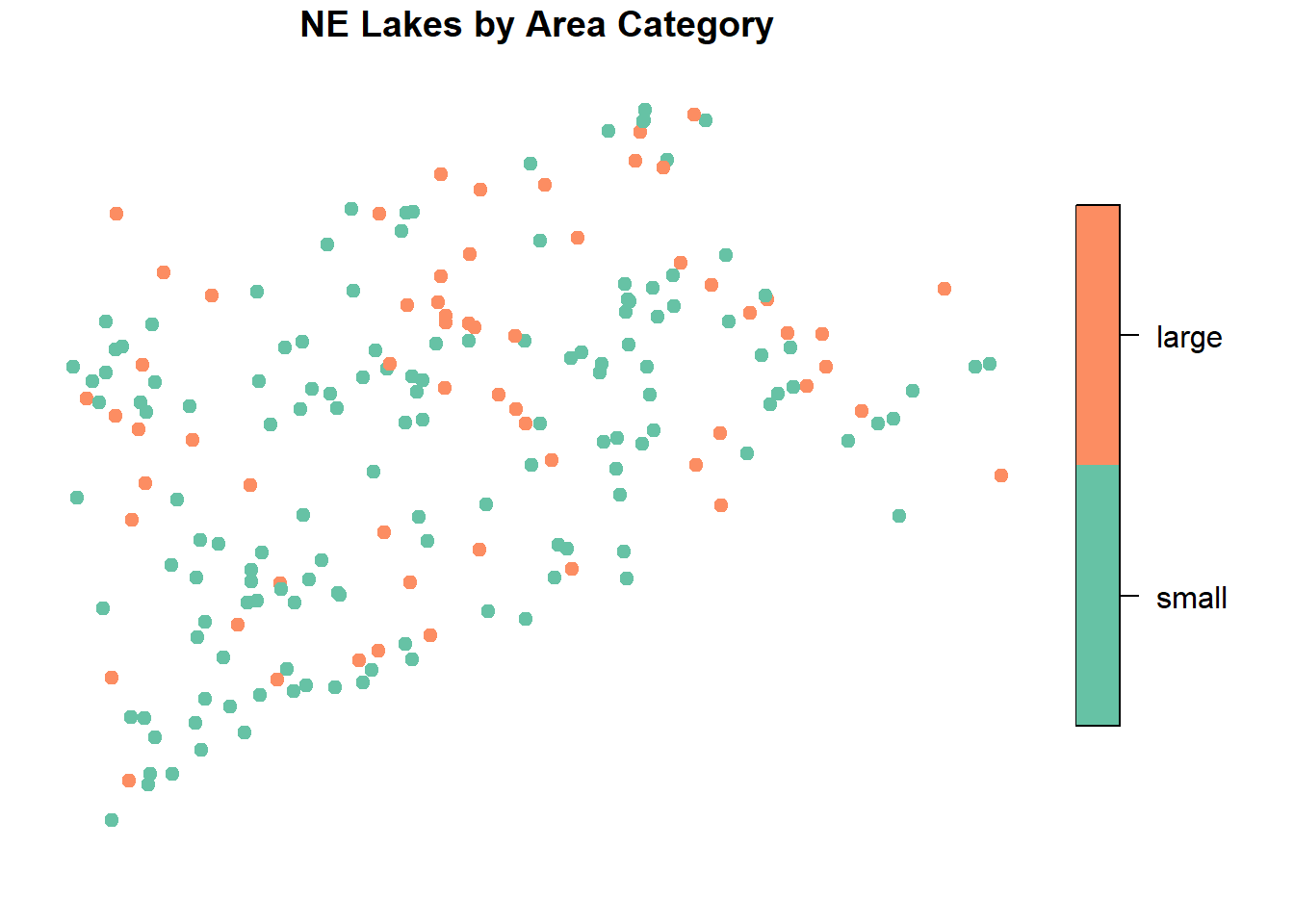
#Plot NE_Lakes stratified by Area Category
plot(NE_Lakes, 
     formula = ~ AREA_CAT,
     main= "NE Lakes by Area Category",
     pch = 19,
     key.width = lcm(3))

propprob <- grts(
  NE_Lakes,
  n_base = 50,
  seltype = "proportional",
  aux_var = "AREA"
)

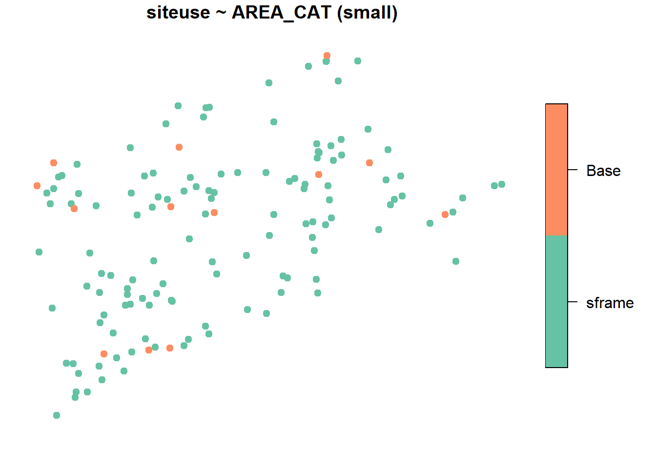
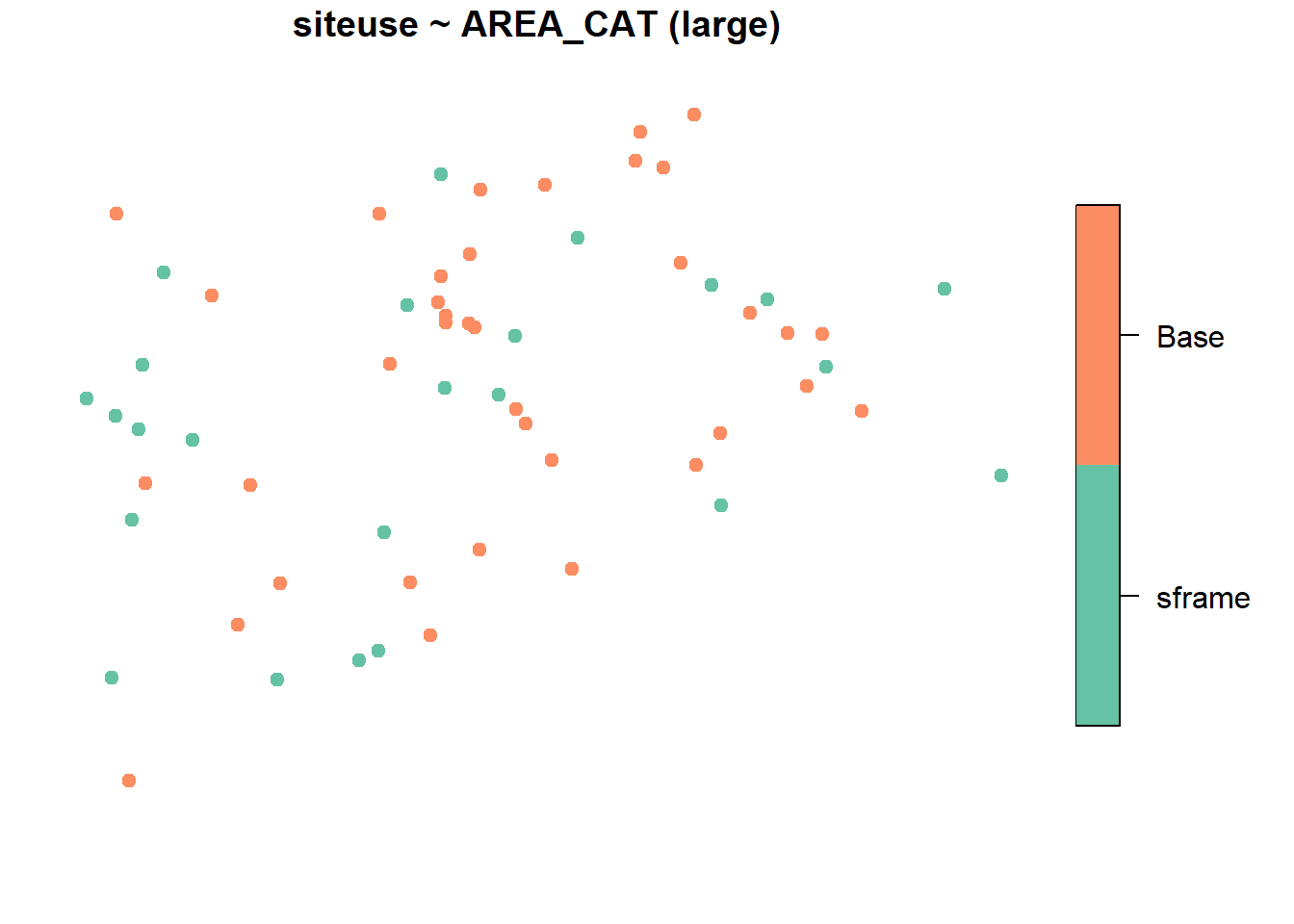
plot(
  propprob,
  formula = siteuse ~ AREA_CAT,
  NE_Lakes,
  pch = 19,
  key.width = lcm(3)
)

10 acres

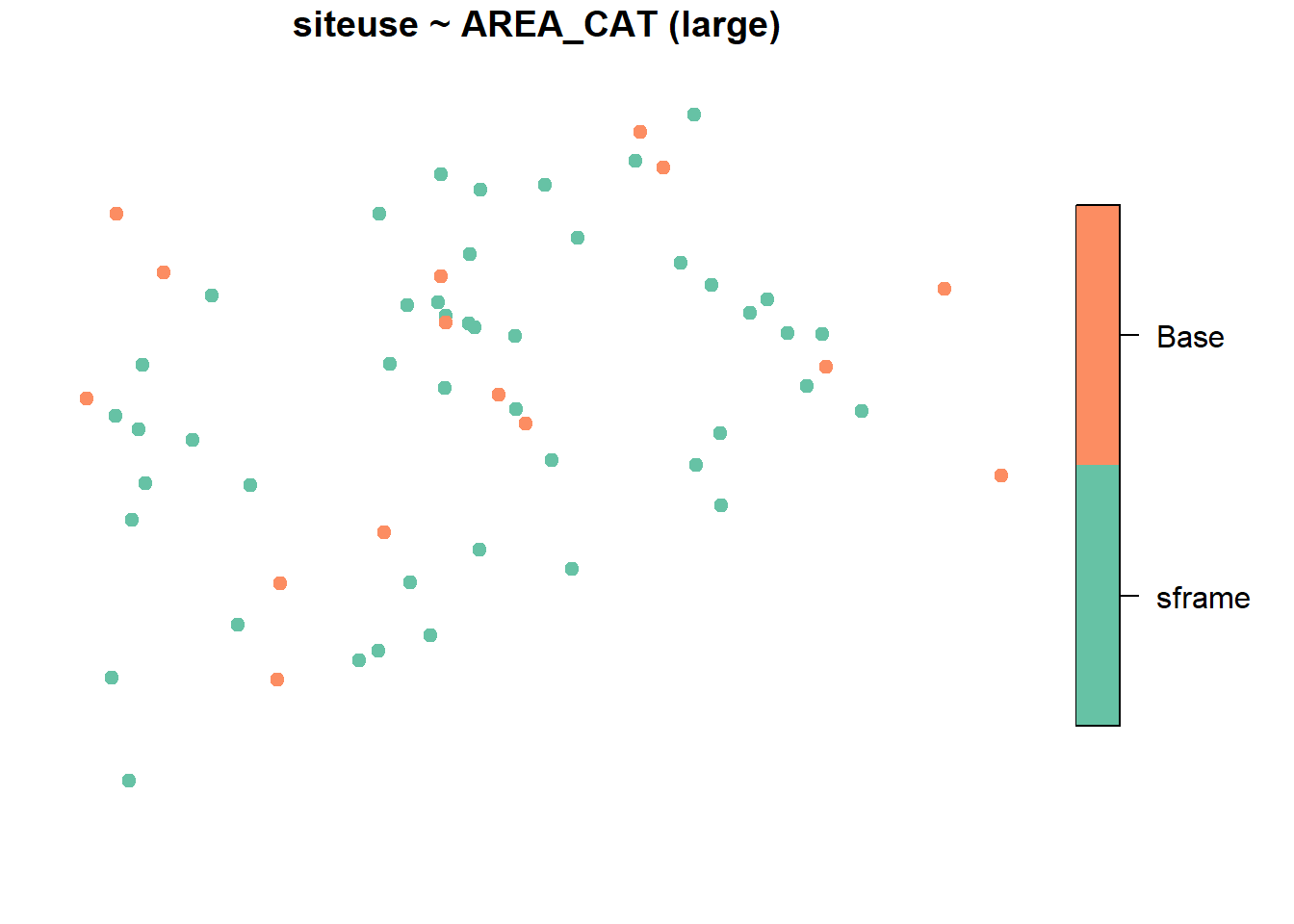
#Create a vector defining stratified sample size
strata_n <- c(small = 35, large = 15)

#Select a stratified GRTS sample 
STRAT_PROB <- grts(
  NE_Lakes,
  n_base = strata_n,
  stratum_var = "AREA_CAT"
)

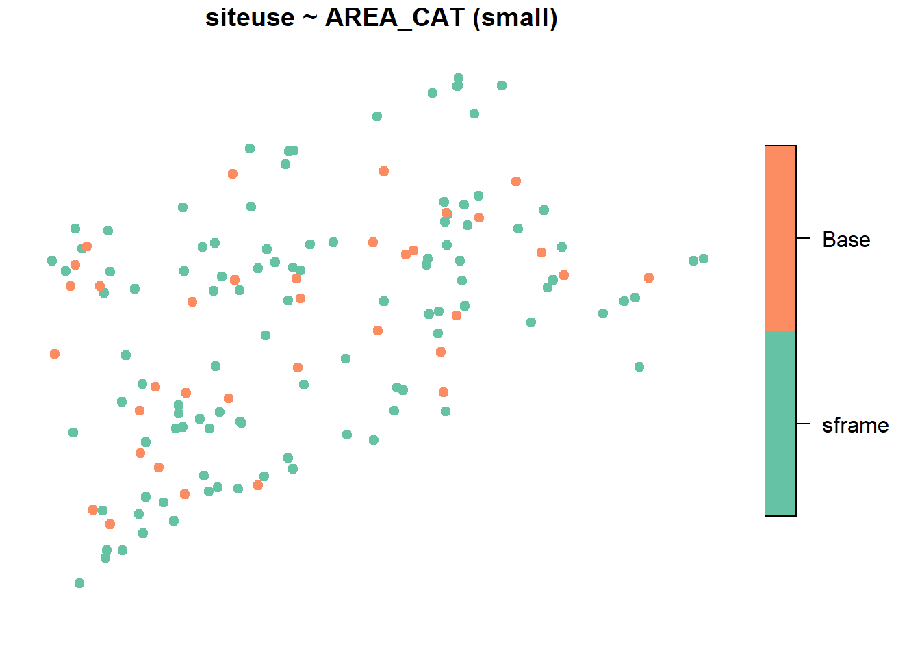
plot(
  STRAT_PROB,
  formula = siteuse ~ AREA_CAT,
  NE_Lakes,
  pch = 19,
  key.width = lcm(3)
)

Background

2 Weights